The System
To demonstrate a planetary rover, the robot had to be integrated into a complete system with computer control and video feedback.
Computer Control
To implement computer control, four main capabilities were needed:
- Read the rover’s joint configurations and calculate the position of its grippers, as well as the orientation of the video system
- Use the thumbwheel switch values of the video subsystem to determine angles to a target in the video frame of reference, and calculate the coordinates of a target in the rover’s frame of reference
- Use the target’s coordinates in the rover’s frame of reference to calculate the joint angles to place a gripper at the target
- Command the rover’s drive tracks, joints, and video system to the desired positions
Joe developed a means to measure each joint’s position by a potentiometer attached to the joint. As a joint moved, the changing resistance of the potentiometer varied a voltage that indicated the position of the joint. The voltage signals from all of the potentiometers were run through a multi-channel digital voltmeter and other circuitry that turned each voltage into a number that could be read by the computer’s input/output system. From the point of view of the computer, the state of the robot’s joints was a list of numbers, one for each joint.
From the computer’s point of view, the robot’s commanded joint positions were another list of numbers. These numbers were sent from the computer to control circuits on the robot.
To control each joint, Joe devised a circuit that accepted the commanded position value from the computer, compared it with the value of the joint’s sensor, and generated a drive voltage for the joint’s motor based on the difference. He designed the circuit so that the drive voltage was constant for large differences, but as the joint’s position neared the commanded position, the drive voltage declined until it reached zero when they coincided. In this way, large movements could be reasonably fast, and yet the joint wouldn’t overshoot its commanded position. (This usually worked well. Occasionally, a joint would overshoot, and then reverse, repeatedly overshooting as it “hunted” for its commanded position.) An incidental advantage of these circuits was that the drive voltages didn’t generate a lot of excess heat in the motors.
I was quite impressed to observe the progress of the modifications to the robot. The entire shoulder/arm systems were disassembled, revealing the drive chains and motors, and the machined surfaces and o-rings that let the hollow arms hold hydraulic fluid under pressure. I don’t recall any leaks when the system was reassembled.
All of the new circuitry was housed in a box mounted on the robot’s base, behind the main post. Another useful feature of the modifications was that they did not disable the use of the manual control panel; either that panel or the new electronics package could be connected to the robot.
Video
The robot originally had no video capability. As a teleoperated device, it relied on the operator’s ability to see the robot and its surroundings, either directly or through a periscope in a blockhouse. To provide for visual inspection and depth perception, a new subsystem was added to the top of the support post. This consisted of a pan-tilt head, driven by the same kind of circuits as the robot’s joints. At the top of this was a cross beam with two identical vidicon tube TV cameras. The two cameras were mounted with their optical axes parallel, and at right angles to the beam. When the pan and tilt positions were zero, both cameras were horizontal and pointed directly ahead. They were spaced about two feet apart. When its “eyes” were installed, the robot was nearly six feet tall.

The robot with pan-tilt head and cameras added. The computer interface electronics is in the box behind the post.
The computer was not powerful enough to process video data. Instead the video signals were sent to two monitors for the human operator to view. Each monitor had a set of cross-hairs superimposed on the screen over the video image, controlled by two three-digit sets of thumbwheels below each screen. The operator adjusted the thumbwheels so that the crosshairs were over a target on each monitor. The computer could not read the thumbwheels; the operator had to type their values into the computer. The software then converted the thumbwheel values to angles from the camera optical axes. Then the computer used the angles from the cameras to calculate the direction and distance to the target. This is why John originally asked Tom to figure out how to compute a target’s position from camera angles.
DEC PDP-1, #13
The computer that was available for this project was from the Digital Equipment Corporation (DEC), and was called the Programmed Data Processor 1 (PDP-1). This was an innovative computer when it was designed in 1959, but the rapid development of computers in the intervening years had made it practically obsolete. DEC only built about 55, and the one we used was serial number 13. Joe told me that it had formerly been used to control a wind tunnel at JPL. By 1972, DEC’s PDP-11 was filling the role formerly performed by the PDP-1.
Recently, I saw a list of PDP-1 serial numbers compiled in 2006 (archived at bitsavers.org) that indicates #13 supported the Ranger program of the early 1960s at JPL, and that #29 supported JPL’s wind tunnel.
The pictures below show an entire PDP-1 computer and a close-up view of its console. Working on this computer, the programmer has to deal directly with the 0’s and 1’s (binary digits, or bits) that underlie all digital computers. The small switches on the console correspond to 0 when down and 1 when up; the lights are on for 1 and off for 0. Nowadays we say this is working “close to the metal.” In those days it was normal.
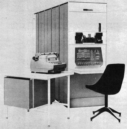
The PDP-1 occupied four refrigerator-sized cabinets, and had a console with an impressive set of switches and blinking lights.
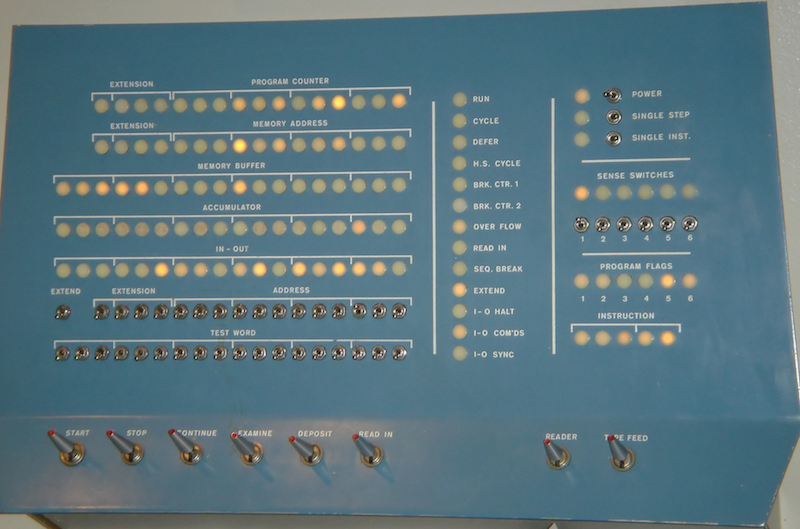
A larger view of the PDP-1’s console, with 119 lights to show the state of the computer, 44 small switches to enter bits into registers, and eight big action switches at the bottom.
The PDP-1 works with “words” of 18 bits (modern personal computers use 64-bit words). The instruction repertoire included logic operations and integer arithmetic, and a relatively rich set of input/output instructions. The machine was well suited to monitoring and controlling laboratory equipment, such as a wind tunnel or the robot. It didn’t have any built-in support for floating-point arithmetic, which was necessary to calculate the trigonometric functions for interpreting the video subsystem and controlling the robot’s arms and gripper.
The PDP-1’s standard method for loading programs into its memory was paper tape. When I started on the project, there was a wicker basket of paper tapes with a variety of utility programs. One of these was called FLINT, for FLoating-point INTerpreter. This was left over from a previous project that involved optics (and “FLINT” was probably a pun on a type of glass used in lenses). A peculiarity of this utility was that it could handle numbers smaller than 1.0 with much greater precision than it could handle larger numbers. This was useful for calculations on angles; it would not have been appropriate for calculations of astronomical distances.
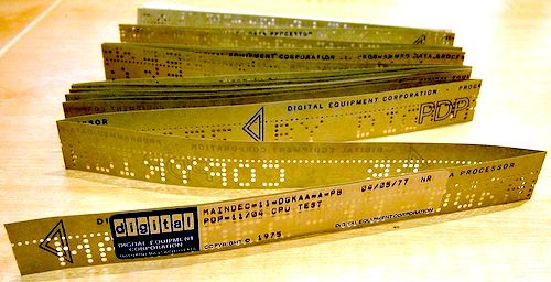
Paper tape similar to the tapes holding the original utility programs that were used with the PDP-1. This is fan-fold tape; rolls of tape were also common. Each hole in the tape corresponds to a 1 (except for the line of small holes down the middle of the tape); the absence of a hole is a 0.
In addition to the paper tape, the computer had an electric typewriter, and three IBM magnetic tape drives, of the kind often seen in old movies to indicate a computer is doing something. One of the utility programs could write a block of the PDP-1’s memory to a magnetic tape, or read a block into memory.
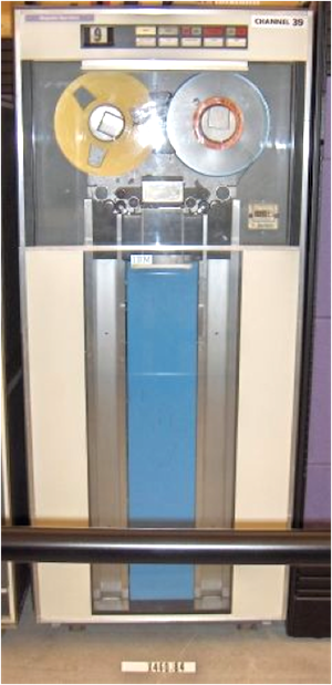
IBM 729 tape drive. The PDP-1 was connected to three drives like this, which needed constant repairs. When reading or writing data, the two reels for the tape spun back and forth in a jerky motion, and loops of tape went up and down the two channels below the reels.
Environment
The space allocated to the project was relatively large and elaborate. In the beginning, it was a single room about 30 feet by 50 feet, with a ceiling at least 10 feet high, and hanging light fixtures. The PDP-1 was at one end, and the robot had a large clear area with a flat concrete floor. The cable connecting the robot to its control panel and power was about an inch thick and at least 30 feet long, with heavy industrial connectors. When I first saw it, the robot’s control panel was sitting on the floor.
Within a few days, a wall was constructed, separating “mission control” (the PDP-1 and TV monitors) from the main demo area. The wall had a large window to view the demo area.
A number of simulated rocks were scattered across the demo area. These were foam rubber with a gray faceted surface that created reflective highlights as they were moved under the overhead lights; they came from a Hollywood prop supply company. The rocks were in a variety of sizes and shapes, typically a few inches across. The robot’s grippers could open up to five or six inches, and easily accommodated them.
Near the PDP-1 console, a second console was set up to hold the two monitors side by side, with the cross-hair thumbwheels below them. Each monitor was about 18 inches across. The two consoles served as our “Mission Control Center” for the demo.
System Diagram
All of these components were integrated into a system, something like the schematic below. (I never saw a system diagram during the project, but if there had been one it would have looked like this.) The arrows show how information flowed through the system. Starting from the robot, the video and robot joint positions were sent to the monitors and computer. The operator used the thumbwheels to identify a target position on the monitors and entered the values into the computer. The computer calculated new joint positions, and sent them to the robot, which then moved to the commanded positions, completing the information flow.
The operator-in-the-loop (me) performed the functions that were beyond the capabilities of the limited computing resources available at the time, such as interpreting the video feed and making decisions.
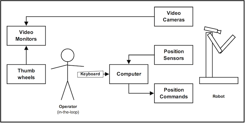
System diagram, showing the robot and the other parts of the system. The operator had to interpret the video monitors, identify the screen locations of a target, and signal the robot to execute each step of the demo scenario.
Next: Part 6 – Demo Scenario